Hamiltonian Tutorial

One of the fundamental goals of quantum chemistry is to elucidate the relationship between molecular structure and properties. Accurate molecular properties can be calculated from the electronic wavefunction, which satisfies the electronic Schrödinger equation. The electronic Schrödinger equation for the system is expressed as Eq. (1). \(|\psi_{el}\rangle\) is the electronic wave-function of the system, \(\hat{H}_{el}\) is the Hamiltonian of the electrons in the system, in the form of equation (2) (atomic units), where \(A\) refers to the nucleus, and, \(i,j\) (i,j refers to electrons.). The first term is the kinetic energy of the electrons, and the second term represents the coulomb attraction between the electron and the nucleus. \(r_{Ai}\) is the distance between electron \(i\) and nucleus \(A\) with atomic number \(Z_{A}\), The third term represents the repulsion between electrons, \(r_{ij}\) is the distance between electron \(i\) and electron \(j\). The solution to equation (1) is based on the assumption that electrons move in the field of fixed atomic nuclei. This approximation holds because nuclear masses in atoms are significantly larger than electron masses, resulting in negligible nuclear motion compared to electronic motion. Consequently, the kinetic energy contribution from nuclei can be omitted, and the electronic motion is approximated by treating the nuclei as stationary.

\[\hat{H}_{el}|\psi_{el}\rangle = E_{el}|\psi_{el}\rangle (1)\]

\[\hat{H}_{el}=-\frac{1}{2} \sum_{i} \nabla_{i}^{2}-\sum_{A,i}\frac{Z_{A}}{r_{A i}}+\sum_{i>j} \frac{1}{r_{ij}} (2)\]

So our core goal can be described as: solving the stationary electron Schrödinger equation in a specific molecular system, obtaining the eigenvalues of the system in different steady-state states, i.e. electron energy. According to the variational principle, the minimum eigenvalue obtained is the ground-state energy of the system \(E_0\) (ground-state energy), The corresponding system state is ground-state.

\[E=\dfrac{\langle \psi |\hat{H}| \psi \rangle}{\langle \psi|\psi \rangle} \geq E_0\]

In the form of second quantization, the electron wave-function can be expressed as an occupation number state, where the orbital order increases sequentially from right to left, as shown in equation (3). Where N is the number of electrons and M is the number of spin orbitals.When the spin orbital \(\chi_p\) is occupied by electrons, \(n_p\) is 1; On the contrary, when not occupied, \(n_p\) is 0. In other words, kets in the occupation basis representation are binary strings with the length of the number of spin orbitals, in which ones define which spin orbitals are occupied. From this, we can apply a series of creation operators to the vacuum state \(|\rangle\) to construct the Hartree-Fock state of any system. As shown in equation (4). In the formula, \(a_{i}^{\dagger}\) is the creation operator, its function is to generate an electron on the i-th spin orbital. Similarly, \(a_{j}\) is defined as the annihilation operator, and its function is to annihilate an electron on the j-th spin orbital.

\[\Phi_{HF}(\chi_1,\chi_2,\cdots,\chi_N)=|n_{M-1},n_{M-2},\cdots,n_0\rangle (3)\]

\[|n_{M-1},n_{M-2},\cdots,n_0\rangle = a_0^{\dagger} a_1^{\dagger} \cdots a_N^{\dagger}|\rangle = \prod_{i=1}^N a_i^{\dagger}|\rangle (4)\]

After second quantization, the Hamiltonian of the electron is expressed in the form of equation (5) [1], the first term in this equation is a one-body operator, the second term is a two-body operator, and the subscript \(pqrs\) represents different electron spin orbitals, where \(h_{pq}\) 、 \(h_{pqrs}\) represents single and double electron integrals, respectively. If the basis set is selected, we can determine the specific value of the integration.

\[\hat{H}_{el}=\sum_{pq} h_{pq} a_{p}^{\dagger} a_{q}+\frac{1}{2} \sum_{pqrs} h_{pqrs} a_{p}^{\dagger} a_{q}^{\dagger} a_{s} a_{r} (5)\]

In pyChemiQ, the molecular Fermionic Hamiltonian can be obtained using the get_molecular_hamiltonian() method. Using the hydrogen molecule (H₂) as an example below, we demonstrate the resulting Hamiltonian.

from pychemiq import Molecules

In the pychemiq.Molecules module, we can initialize molecular electronic structure parameters, including geometry (with coordinates in angstroms), basis set, charge, and spin multiplicity. The molecular information is stored as an object, and classical Hartree-Fock calculations are executed after input parameters are provided.

multiplicity = 1
charge = 0
basis =  "sto-3g"
geom = "H 0 0 0,H 0 0 0.74"
mol = Molecules(
    geometry = geom,
    basis    = basis,
    multiplicity = multiplicity,
    charge = charge)

By calling get_molecular_hamiltonian(), we can obtain the molecular Hamiltonian sub-terms in Fermion form and the coefficients of each term. The following is the example code and the printed results of the fermionic Hamiltonian for hydrogen molecules.

fermion_H2 = mol.get_molecular_hamiltonian()
print(fermion_H2)

{
: 0.715104
0+ 0 : -1.253310
1+ 0+ 1 0 : -0.674756
1+ 0+ 3 2 : -0.181210
1+ 1 : -1.253310
2+ 0+ 2 0 : -0.482501
2+ 1+ 2 1 : -0.663711
2+ 1+ 3 0 : 0.181210
2+ 2 : -0.475069
3+ 0+ 2 1 : 0.181210
3+ 0+ 3 0 : -0.663711
3+ 1+ 3 1 : -0.482501
3+ 2+ 1 0 : -0.181210
3+ 2+ 3 2 : -0.697652
3+ 3 : -0.475069
}

In addition, pyChemiQ supports the configuration of active spaces and frozen orbitals. By restricting both the electrons and the orbitals involved in excitations, the method considers only specific electron excitations to designated orbitals. Proper application of active spaces and frozen orbitals reduces the required number of qubits for simulation while maintaining chemical accuracy.

The active space method (equivalent to CASSCF in classical quantum chemistry) divides molecular orbitals into three categories: - Doubly occupied orbitals (permanently filled with two electrons) - Active orbitals (where limited electrons undergo configuration changes) - Virtual orbitals (permanently unoccupied) Electrons are confined to undergo configuration changes only within the active orbitals. An active space is denoted as [m,n], where m represents the number of active orbitals and n the number of active electrons. This formulation accounts for all possible configurations of n electrons distributed across m orbitals. Active orbitals are typically selected around the HOMO and LUMO regions, as electrons in these orbitals—comparable to valence electrons in atomic orbitals—are the most chemically reactive and drive chemical transformations. Below is an example of the [2,2] active space:

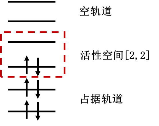
Figure 1: Partition of molecular orbitals in active space setup

In pyChemiQ, the active space is specified via the active parameter within the pychemiq.Molecules module. For example, to obtain the Hamiltonian for LiH using a [2,2] active space:

multiplicity = 1
charge = 0
basis =  "sto-3g"
geom = ["Li     0.00000000    0.00000000    0.37770300",
        "H      0.00000000    0.00000000   -1.13310900"]
active = [2,2]
mol = Molecules(
    geometry = geom,
    basis    = basis,
    multiplicity = multiplicity,
    charge = charge,
    active = active)
fermion_LiH = mol.get_molecular_hamiltonian()

The setting of pyChemiQ for the number of frozen orbitals is specified through the ‘nfrozen’ parameter. By default, we start freezing the orbitals and their electrons from the lowest-energy molecular orbitals. For example, in the following example, we freeze a space orbital to obtain the Hamiltonian of LiH:

multiplicity = 1
charge = 0
basis =  "sto-3g"
geom = ["Li     0.00000000    0.00000000    0.37770300",
        "H      0.00000000    0.00000000   -1.13310900"]
nfrozen = 1
mol = Molecules(
    geometry = geom,
    basis    = basis,
    multiplicity = multiplicity,
    charge = charge,
    nfrozen = nfrozen)
fermion_LiH = mol.get_molecular_hamiltonian()

References

[1]

Attila Szabo and Neil S Ostlund. Modern quantum chemistry: introduction to advanced electronic structure theory. Courier Corporation, 2012.